Making 1M Click Predictions per Second using AWS

Written by Chris Evans, April 26, 2018

Click prediction may be a simple binary classification problem, but it requires a robust system architecture to function in production at scale. At AdRoll, we leverage the AWS ecosystem along with a suite of third party tools to build the predictors that power our pricing engine, BidIQ. This is a tour of the production pipelines and monitoring systems that keep BidIQ running.

Introduction

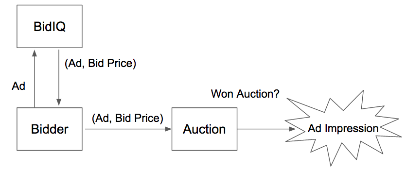
AdRoll participates on Real Time Bidding (RTB) exchanges to display ads for our advertisers. When a user visits a website, a real-time auction takes place while the page loads. AdRoll submits an ad and a bid price, and if our bid wins, our ad is displayed.

In more detail, AdRoll has a number of machines we call “bidders,” which are integrated to the various ad exchanges which run RTB auctions. These exchanges send “bid requests” to our bidders. For each bid request, our bidders determine a list of ads we might show and for each ad, our bidders query BidIQ, our pricing engine, to determine what price we are willing to bid for it. Then the bidders take the ad with the highest bid price and send it to the exchange.

The Data Science Engineering team works on BidIQ and the loose coupling between the bidders and BidIQ gives us complete flexibility in how we price each ad and what infrastructure we use. BidIQ determines the bid price for an ad based on the advertiser’s campaign goals and a series of models that predict the probabilities that the ad will be viewable, that the user will click our ad, and that the user will go on to take an “action” (e.g. buy something), among others.

In this blog post I’ll focus on BidIQ’s click predictor, which we built first and have used the longest. When I tell people familiar with machine learning about it, they are often skeptical that there is much to do: “Isn’t that just a binary classifier?”

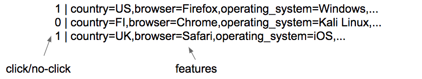
Indeed click prediction is a classic binary classification problem. We can build a dataset with one line for each impression (displayed advertisement), labeled 1 or 0 according to whether it was clicked or not, along with a list of features (time of day, geographic location, etc.) for that impression. Then for a fresh impression, our problem is to predict how likely it is to be 1 based on its features.

Now standard machine learning approaches apply. We can split the dataset into a train and test set, choose a subset of features, train a logistic regression on the train set, evaluate it on the test set, and repeat with different subsets of features until we find the subset which minimizes the average log-loss on the test set. Then, after training a model with the selected subset of features over the whole set of data, we can use it to make click predictions for future ads.

Were this a textbook exercise, we’d be done, yet we are just getting started. This is where the “Engineering” in Data Science Engineering comes in.

For our production system we need to:

• Automate everything: training set generation, model training, model deployment, and updates
• Update models frequently, and with zero downtime; we need to price ads 24/7
• Handle a throughput of one million queries per second, responding to each with less than 20 milliseconds of latency
• Facilitate model improvements and feature discovery by our engineers in parallel
• Allow multiple live A/B tests of different models
• Monitor our production pipeline carefully as well as the inputs and outputs of the model

To build our system architecture satisfying these requirements, we use the AWS ecosystem heavily as well as a variety of third party and open source tools. A list of these tools and their descriptions is in the Appendix.

Training The Model

There are three steps in our training pipeline:

1. Generate the training dataset
2. Train a model against the training dataset
3. Wrap the model with serving code in a docker image for easy deployment

We handle these steps with Docker, AWS Batch, and Luigi.

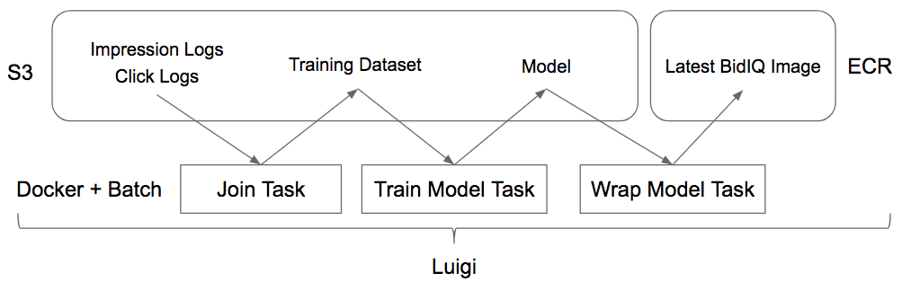
Our starting point is the impression and click logs our bidders generate and store on S3.

For step one, we’ve built a Docker image which takes a time range, downloads the impression and click logs in that time range, joins them, and uploads the resultant dataset to S3.

To generate the model, we’ve built a Docker image which takes a time range and model configuration, downloads the training dataset in that time range, trains a model against the dataset, and uploads it to S3.

Finally, we download the model, combine it with serving code in a Docker image, and upload it to our ECR repository. This final image can then be easily deployed to any EC2 instance where it can price queries on a specified port.

These tasks are placed in a Luigi pipeline and kicked off via AWS Batch when the upstream requirements are satisfied. This ensures that freshly generated logs are joined and incorporated into our most recent model with minimal delay and computing resources.

Deploying and Updating the Model

Model Deployment

AdRoll displays ads to users all over the world. Given the tight latency restrictions of RTB, we’ve placed our bidders all over the world as well. More concretely, our bidders run on EC2 instances in multiple AWS regions. Thus, in order to keep the latency between the bidders and BidIQ under 20ms, we also need to deploy BidIQ servers in each AWS region. Furthermore, in each region we may need BidIQ servers for multiple versions of the model (e.g. for A/B tests).

Architecturally, we handle this by having one Auto Scaling Group (ASG) per (BidIQ Version, AWS Region) pair. Then, by changing the size of the ASG, we can trivially scale up or down the throughput of ad auctions that BidIQ can price. For example, we can scale down BidIQ versions which are only tested on a small percentage of traffic or scale up heavily trafficked AWS regions.

We use Terraform to manage the deployment of the BidIQ ASGs and store the generated .tfstate files on S3, sharded by BidIQ version and AWS region. In this way, any engineer can easily deploy or modify the ASG for a given (BidIQ Version, AWS Region) with a simple terraform apply.

Service Discovery

So now we have BidIQ ASGs serving the model, and bidder instances which need to query the model. How can the bidders know which host and port to query to reach a given BidIQ version?

For this we use a DynamoDB table called Services. We have one such table per AWS region, and each BidIQ instance in that region announces itself on that table. The BidIQ instance periodically heartbeats an entry to the table consisting of:

HOST, PORT, BIDIQ_VERSION, EXPIRY_TS

BidIQ upholds the contract:

1. Each (HOST, PORT) can be queried for that BIDIQ_VERSION until the current time exceeds EXPIRY_TS.
2. For each BIDIQ_VERSION there will be sufficient (HOST, PORT) tuples to meet throughput. To guarantee this, BidIQ ensures both:
   • For each HOST, at least one PORT is available
   • We have sufficiently many HOSTs for the given BIDIQ_VERSION

Model Updates

Our pipeline is constantly pushing updates to the model as more recent data come in. We need to swap in these fresh models while upholding the contract above.

To do this, each instance in the BidIQ ASG uses the following logic, orchestrated by a Python script:

• Every five seconds, query the locally running model as a health check. If this health check fails, restart the model.
• Every minute, check for an updated model. If found:
  1. Download the new model and run it on a new port
  2. Start heartbeating the new port to the Services table
  3. Stop heartbeating the old port to the Services table
  4. After a grace period for draining, shut down the model on the old port

This logic is simple, allows for smooth model updates with no down time, and requires no coordination between individual instances in a BidIQ ASG. And our bidders don’t need to know anything about the internals of BidIQ. They simply look up a (HOST, PORT) in the Services table for a given BIDIQ_VERSION and query it to get a bid price.

Improving the Model

I’ve explained how we handle model updates for a given version of BidIQ, but how do we improve the model to make new versions of BidIQ? Model improvement is broken into two phases, Backtesting and live A/B testing.

Backtesting

For backtesting new models, we have a simple web application, “Juxtaposer”. A user can define an experiment via a YAML configuration consisting of which versions of our code to use, what features to use in the model, which train and test sets to use, and even the Docker image to run the experiment in.

We then kick off this dockerized experiment via AWS Batch. When finished, it reports metrics back to the web app, where we can compare them side-by-side (hence the name “Juxtaposer”). With Docker and AWS Batch it is trivial to kick off an arbitrarily large number of experiments in parallel, and our engineers can focus on improving the model without worrying about infrastructure.

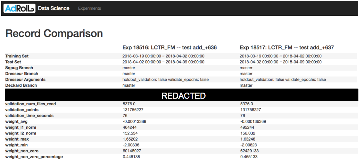
For feature engineering, we typically look at standard binary classification metrics (average log-loss, AUC, etc.) on the test set, whereas for changes to our code, we look out for regressions—backtesting gives us a dry run of how the model will behave in production.

Live A/B Testing

Once we have a new model that looks good in backtesting, we A/B test it live. For this we use Collider. In a nutshell, Collider instructs the bidders to apply custom logic to a fixed percentage of live traffic. For our purposes, we simply tell the bidders to use a specified BIDIQ_VERSION rather than the production version.

For A/B testing, in addition to binary classification metrics, we look at broader ad-tech metrics such as our observed cost-per-click (CPC) or cost-per-action (CPA). If the test version of BidIQ looks good we roll it out as the new production version.

Monitoring our Production Model

With the great power of BidIQ (pricing one million ads per second, each within 20ms, 24/7) comes great responsibility: BidIQ is an automated system which controls how we spend money so it is imperative that we monitor it closely, especially as much of the data it ingests comes from ad exchanges, which may introduce changes outside of our control.

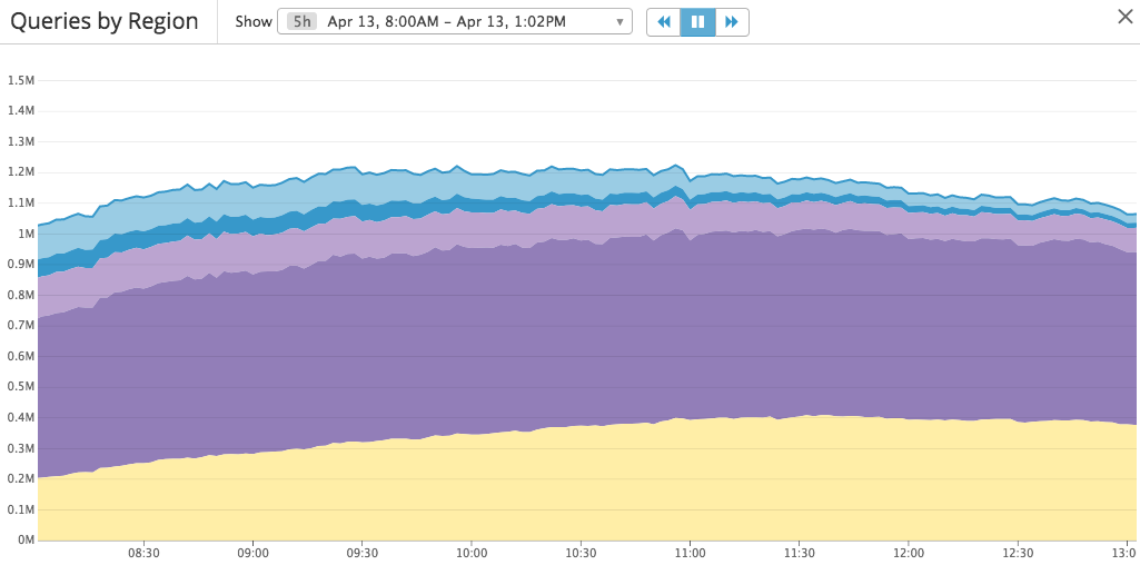
To start, we use Datadog for real-time monitoring. Each BidIQ server outputs simple metrics in UDP packets, using the StatsD protocol, which are picked up by a local Datadog agent, aggregated, and displayed in a real-time dashboard. In this way, we can see our live average predictions and average bids across a number of dimensions and send a Pager Duty alert if something suddenly changes.

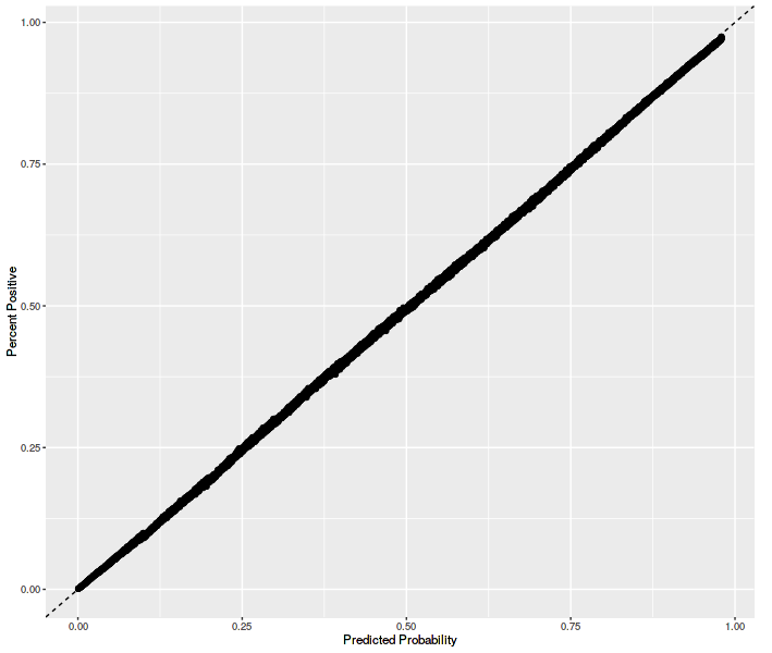
Next, our bidders log the bid prices and click predictions that BidIQ returns in our impression and click logs on S3. Using Presto, we can easily query these logs with SQL. With some simple SQL queries we can check, on various subsets of traffic, whether the ratio of expected clicks (sum of click-probabilities over impressions) to actual clicks is close to one, as it should be. With slightly more complicated queries we can build calibration curves to verify that our predictions have been accurate.

Next, we expose our joined training logs to Presto so we can directly query the data BidIQ is ingesting. We also have a script that taps our live BidIQ servers (using tcpdump) to see exactly what data our bidders are sending them. These have proven invaluable in investigating changes in upstream data.

Next, most of our tasks deliver email messages on failure, and our task to train the model runs additional sanity checks to ensure that parameters such as average prediction over the test set are within reasonable bounds. We also have a catch-all monitoring repository, “Night’s Watch,” which contains a series of Python scripts which send us warning emails if anything is off (e.g. a BidIQ model hasn’t been updated recently).

Finally, each of our code repos has a thorough set of unit and integration tests.

Conclusion

Hopefully the above gives you a sense of the architecture and infrastructure involved in bringing even a simple binary classifier into stable production at scale.

And that’s just our high-level architecture. With our predictors being so critical to our business, we’ve written custom code to train and serve our models in a low-level language, D. We’ve optimized our D code for our use cases: we’ve disabled garbage collection (violates our latency requirement), removed any allocations on the heap, rewritten performance bottlenecks using intrinsics, added logic to price a batch of ads at a time with multithreading, and more. And on the algorithm side, we now use an extension of logistic regression, factorization machines.

So far we’ve only discussed our click predictor. We have a number of other predictors with their own quirks as well as an ever-evolving set of logic to choose a bid price in the face of evolving auction dynamics, notably the recent rise in header bidding.

The best thing about working on Data Science Engineering at AdRoll is that you work at the intersection of so many interesting fields: math, statistics, computer science, machine learning, computer networking, economics, game theory, and even web development. Most of our projects overlap with a number of these fields, and our team has a diverse group of engineers with backgrounds across these fields so there is always something new to learn and someone to learn from. We are regularly looking for new engineers so if these areas interest you, let us know!

Appendix

List of AWS tools we use

• ASG – scalable group of EC2 instances
• Batch – easy way to run a docker image
• DynamoDB – low latency NoSQL database
• EC2 – on-demand machines to run our code
• ECR – repo for docker images
• S3 – cloud storage for flat files

List of third party / open source tools we use

• Datadog – reporting for live metrics
• Docker – simple containerization
• Luigi – simple pipeline logic to kick off jobs once upstream ones finish
• Pager Duty – alarm system to alert engineers when something goes wrong
• Presto – fast SQL query engine which can also query large csv files on S3
• Terraform – simple declaritive language to create and modify AWS infrastructure

Do you enjoy designing and deploying machine learning models at scale? Roll with Us!